1. Introduction

 

The Gulf of Guinea region in Africa is a vague area of contiguous maritime and continental space along the West African coast. In terms of oil geopolitics, some authors limit the Gulf of Guinea to the oil-producing countries along the West African coast, stretching from Côte d'Ivoire to Angola (Kounou 2009). This zone is characterized by the abundance of natural resources, particularly oil (Ndoutoume 2010). The economies of these countries heavily rely on oil exploitation. For example, in 2000, the oil production of the Gulf of Guinea countries accounted for approximately 3.8 billion tons, representing around 5% of global production. The good quality of its crude oil attracts the interest of numerous investors (Amoussou 2018).

 

The intensification of oil activities in this region leads to an increase in anthropogenic activities, resulting in oil spills. Analysis of some studies in the field shows that between 2002 and 2012, the Republic of Congo had a high probability of hydrocarbon spills, following Nigeria and Cameroon (Amoussou 2018). Similarly, Ngoma (2015) shows that the Democratic Republic of Congo (DRC) experienced extensive hydrocarbon spills between January and April 2010. In Gabon, particularly at the Cap Lopez terminal (Port-Gentil), an incident in 2022 due to a storage tank leak resulted in an oil spill of approximately 50,000 cubic meters (Malouana Biggie 2022). These cases highlight the extent of the pollution problem related to oil exploitation in this region. It is important for scientists to guide decision-makers toward suitable solutions that would help strengthen the region's legislation. In addressing this issue, we believe that the use of remote sensing can monitor the expansion of oil spills in marine environments. The use of Earth observation tools, especially SAR imagery, appears to be a potential avenue for identifying and mapping areas with high oil pollution.

To construct our reasoning, we relied on the approaches detailed by Najoui (2017) in his literature review. In his work, she explains that the detection of marine oil slicks includes four basic steps: 1) images preprocessing, 2) dark patches segmentation, 3) features extraction and 4) oil slicks classification (Solberg et al. 1999; Brekke and Solberg 2005; Topouzelis and Konstantinos 2008). Generally, in the literature, the image preprocessing (first step) is limited to speckle filtering on standard detected products. Unfortunately, so many heterogeneities remain in the radar images after such classical preprocessing hindering the "robustness" of the segmentation and the classification methods especially when working on large areas. The work of this paper focuses on image preprocessing and dark patches segmentation. Due to the incidence angle dependencies (SAR images tend to become darker with increasing range), upwind/downwind or crosswind, and swath width effects, brightness variations may occur in the SAR images and hence compromise the processing of SAR images. A variety of segmentation methods have been proposed and are listed below: adaptive thresholding (Solberg et al.1999), hysteresis thresholding (Kanaa et al. 2003), edge detection using Laplace of Gaussians or Difference of Gaussians (Chang et al. 2008), wavelets (Liu et al. 1997), mathematical morphology (Gasull et al. 2002), neural network (Garcia-Pineda et al. 2009; Angiuli et al. 2006; Del Frate et al. 2013), etc., etc. Even though a variety of segmentation methods have been applied, the most frequently used are based on a local analysis to overcome the brightness variations in the SAR images. In the study area, scientific work on the detection of oil slicks at sea by remote sensing is virtually non-existent. Previous studies have investigated the pollution problems (Kounou 2009; Malouana 2022; Mbaki 2003) and mapped local oil slicks in the Gulf of Guinea area (Najoui 2017; Najoui 2022a; Najoui 2022b; Najoui 2018a; Najoui 2018b; Okafor 2018). However, to our knowledge, this study is the first to carry out a statistical analysis followed by the proposal of a first intelligent GIS approach capable of monitoring the evolution of slick drift followed by their change of state. This work aims to evaluate particularly in the areas of the two Congos and Cabinda (Angola) from 2015 to 2020. Our methodology is based on the pre-processing of radar images to facilitate the semi-automatic detection of oil slicks and then to make the semi-automatic recognition of marine oil slicks more reliable. The main objective is to implement an intelligent GIS for data prediction and analysis. In this article, we will present the materials and methods section, followed by the presentation and discussion of the results in section 3. Finally, we conclude with some perspectives.

 

2. Study area

 

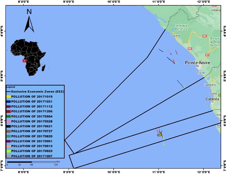
The study area of this work is located at the confluence of three countries: The Republic of Congo, the Democratic Republic of Congo (DRC), and the Republic of Angola through its Cabinda region. Regarding the Republic of Congo, it is situated in the center of Africa in the coastal zone. This country spans 162 km of coastline, featuring bays and points such as Pointe Noire, Indienne, and Kounda. The map below (Figure 1) illustrates the selected study area for this work.

 

 

 

 

 

 

 

 

 

 

 

 

 

 

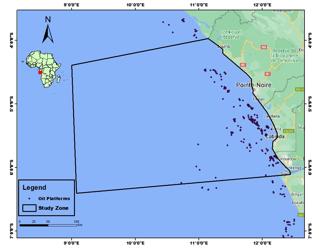
It specifically covers the maritime frontage of both Congo and Cabinda. This region is of particular interest for several reasons, as it is situated at the convergence of three oil-producing countries in a confined space and hosts multiple oil platforms.

 

3. Methodology

 

The analysis of radar images for hydrocarbon slick detection has been the subject of several studies. Generally, three approaches emerge: a manual approach conducted by trained human operators who analyze the images to detect hydrocarbon slicks. This approach is very rare. The semi-automatic approach where a computer detects all black objects in the radar image using various segmentation techniques, after which an experienced human operator classifies these objects as oil slicks or look-alikes. Finally, the automatic system that uses complex image processing and programming techniques to perform both segmentation and classification. In our case, we have opted for the semi-automatic approach considering the software tools at our disposal.

   

3.1.Downloading

 

The collection of Sentinel-1 data was carried out on the ASF Data Search platform. This platform is a satellite data archiving platform developed by the University of Alaska's Institute of Geophysics and managed by National Aeronautics and Space Administration (NASA). The choice of this sensor is explained by the fact that it covers the period 2015 to 2020, which is the subject of our study. This is not the case for Sentinel 1B, which was put into orbit in 2016. Also, on the download platform Sentinel 1B did not have all the data we needed. Downloading the data is free for all users. We proceeded with downloading the data for the period from 2015 to 2020. This data acquisition step allowed us to collect approximately 644 Sentinel-1A sensor data on a day-to-day basis over the 6 years. Table 1 below shows the data parameters.

 

 

CHARACTERISTIC	DATA TYPES
Number of data collected	565
Mission	SENTINEL 1_A
Period	2015-2020
Acquisition mode	IW
Product type	GRD
Direction	ASCENDANT
Polarisation	VV , VH
Instrument name	C-band synthetic aperture radar
Swath	250 Kilometers
Resolution	5X20 meters

 

3.2.Data pre-processing

 

The downloading step was followed by a data pre-processing phase. This phase aimed to enhance the perception of certain details present in each of the images. The software used for these treatments was SNAP. Several reasons guided us in choosing this software: its free accessibility, its ability to perform quick pre-processing, and its reliability in detecting dark spots in radar imagery. The pre-processing step was preceded by a phase that involved reducing the sizes of the images. Indeed, with a Swat of approximately 250 km and a resolution of 5 meters by 20 meters, the size of the images was very high. This situation made the pre-processing phase very challenging. Faced with this difficulty, we created sub-images taking into account the areas of interest. This step facilitated the processing time of the algorithms.

After this step, we moved on to the pre-processing phase. This process unfolded in the following steps: calibration, ellipsoid correction, multilook, land-sea mask application, conversion to decibels, and speackle filter. The complete description of these steps is as follows:

 

· Calibration: It consisted of obtaining values at the level of the images which are representative of the target surface sought.

· The multilook process, on the other hand, helped reduce the speckled effects on the images, which hinder the visualization of all the information present in each image. For this step, we utilized the multilook tool. This tool allows for the combination of multiple images incoherently, as if they corresponded to different views of the same scene. The multilook tool has the effect of improving the image interpretation process and enhancing the execution of the speckle filter.

· The ellipsoid correction was applied to ensure that the representation of the processed image in SNAP is as close as possible to the reality on the ground. The land-sea mask tool was used to mask terrestrial data and represent the entire marine domain of the target area.

· The speackle filter was used to mitigate the overall noise or shimmer present in the raw images. This noise can disturb the perception of objects or the detection of dark spots in the image. This process aims to highlight dark spots and contextual elements by reducing unwanted interference.

· The conversion to decibels: was used to better visualize oil slicks and differentiate them from their look-alikes. We performed a reading of the processed image in decibels. This enhances the contrast of the image and characterizes the intensity across the entire image. Each area of the image corresponds to a specific intensity, which is high or positive in brighter areas and low or negative in darker areas. Through this conversion, one can read in decibel values the echoes recorded by the radar sensor. This recorded echo is representative of the backscattering intensity and the behavior of electromagnetic waves when interacting with the target area.

 

Following the pre-processing in SNAP, we identified areas with a high presence of oil slicks solely of petroleum origin. However, some look-alikes may resemble hydrocarbon slicks with the same spectral signature. Depending on the look-alikes, the backscattering intensity in decibels read on the radar image after conversion varies. Generally, upon observation, only certain look-alikes, such as biological slicks, often exhibited spectral signatures quite similar to those of hydrocarbon slicks. However, we eliminated them since they typically develop in clusters, far from oil platforms. After this work, we proceeded to save the results in GeoTIFF format, which is useful for future processing with QGIS software.

 

3. Data processing

 

After the pre-processing phase, we exported all the data to the Quantum GIS (QGIS) software for the digitization of detected pollution. In total, we identified and digitized 244 hydrocarbon slicks. This digitization led to the creation of vector data, which were subsequently classified by acquisition date. Next, the calculation of the areas of each vector's attributes was performed. The attribute data of each vector were then exported to a spreadsheet for the creation of various graphs. The last phase of these treatments was the production of an annual map of hydrocarbon pollution slicks. Figure 2 below schematically describes all the aforementioned steps.

Small image production phase

 

Calibration and correction phase

Application of the multilook

Application of the speakle filter

Digitization phase

Production of vectors

Production of an intelligent GIS

Derivation

Prediction

Statistical analysis

Downloading images

Application of the Land Sea Mask

Linear to DB

 

 

 

 

 

 

 

 

 

 

 

 

 

 

 

 

 

 

 

 

 

 

 

 

 

 

 

 

Following the presentation of the methodology, we will now detail the results of our treatments.

 

4. Results

The results we present below are the result of processing several data mainly from 2 zones. the table below summarises all the data used year after year. The data used in this study are summarised in Table 2 below.

	2015	2016	2017	2018	2019	2020	total
Area 1 : Cabinda-RDC	15	19	45	72	57	61	269
Area 2 : République Congo	13	16	90	56	60	61	296
Total	28	35	135	128	117	122	565

 

 

 

 

 

 

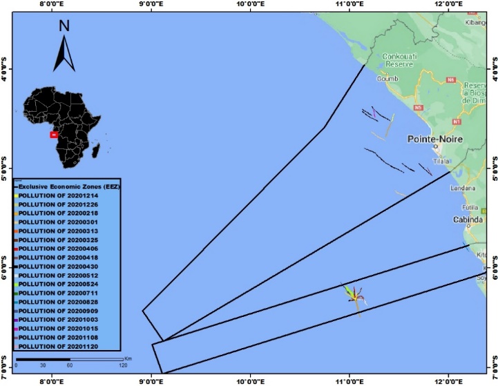
The mapping of oil slicks was carried out step by step over the selected 6 years. The oil slicks were mapped step by step over the six years selected. Each figure (3 to 8) shows the slicks detected after elimination of look-alikes. To achieve these results, we used Bragg's theory. The wave emitted by a surface with irregularities is equal to half the wavelength of the incident wave. In the case of look-alikes, and depending on the irregularities of the sea surface, the intensity in decibels can vary between -26 and -29 dB. In the case of oil slicks and biological slicks, due to their viscoelastic properties, this intensity can vary between -22 and -24 dB. However, biological slicks develop in agglomerations, which differentiates them from oil slicks. To remove any doubts about slick detection, we based our analysis on the contextual elements of the image, in particular the oil platforms associated with each slick detected. In addition, in order to rule out similarities in the radar image, we relied on the differences in the shape, texture, extent, etc. of the oil slicks. In addition, in order to exclude similarities in the radar image, we relied on the differences in shape, texture, extent, etc. of the oil slicks. In addition, in order to exclude similarities in the radar image, we relied on the differences in shape, texture, extent, etc. of the oil slicks. The maps below show the spread of oil slicks from 2015 to 2020 (Fig. 3). The maps in Figure 3 below show the different oil slicks from 2015 to 2020. In A we have the situation in 2015, B in 2016, C in 2017, D in 2018, E in 2019, F in 2020.

 

                                         A                                                                             B

 

 

 

 

 

 

 

 

 

 

 

 

 

 

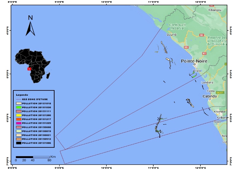
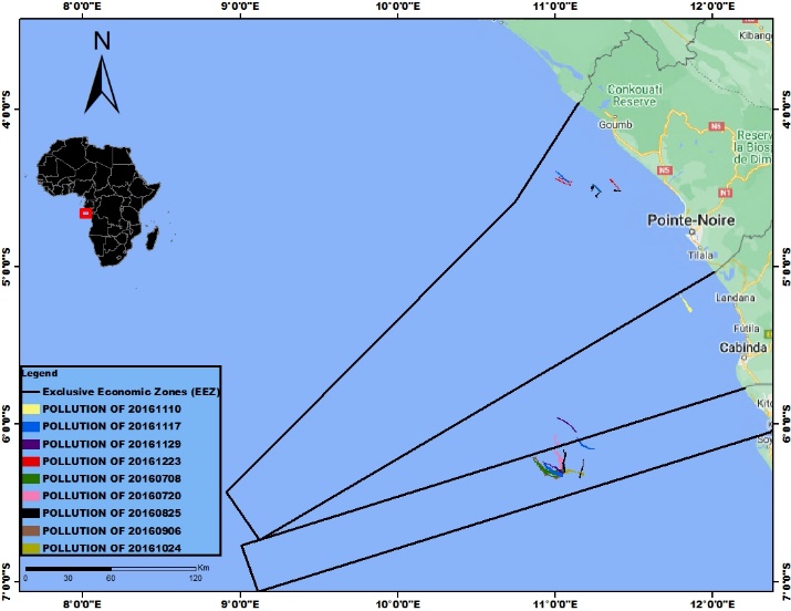
                               C                                                                                    D

 

 

 

 

 

 

 

 

 

 

 

 

 

 

 

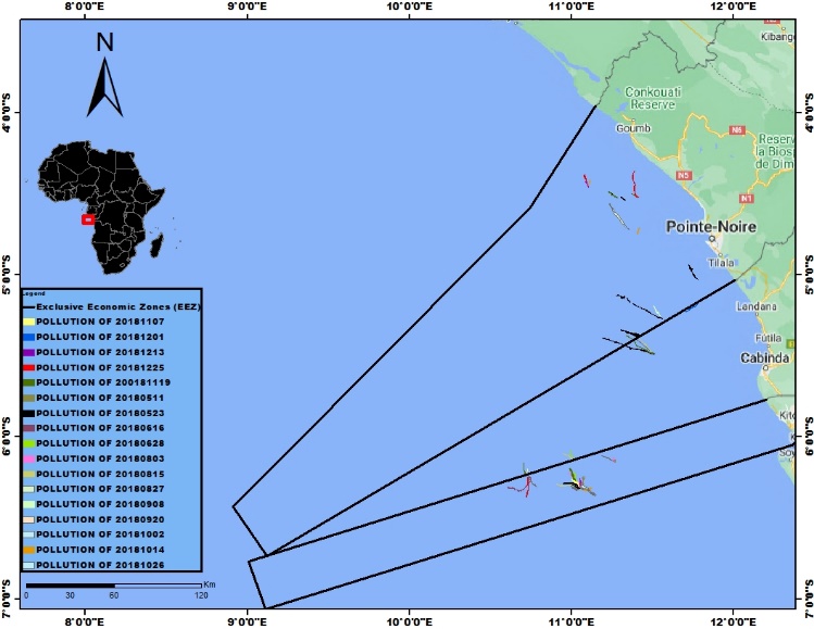
                                          E                                                                         F

 

 

 

 

 

 

 

 

 

 

 

 

 

 

 

After the mapping work from 2015 to 2020, we have summarized all of these results through the table below. Table 3 gives a breakdown by year of the quantity of slicks detected.

 

Year	CB	DRC	Cabinda	Total
2015	23	22	19	64
2016	17	17	2	36
2017	17	12	3	32
2018	13	24	8	45
2019	14	16	4	34
2020	12	24	0	36
Total	96	115	36

 

From this identification work, we subsequently calculated the pollution surfaces at the water tables. Table 4 shows the surface area in km² occupied by groundwater per year.

 

Year	CB	DRC	Cabinda	Total
2015	132,984	113,47	57,987	304,441
2016	35,032	156,006	15,923	206,961
2017	58,754	93,114	8,056	159,924
2018	50,438	106,464	42,171	199,073
2019	28,82	104,961	2,937	136,718
2020	52,882	131,71	0	184,592
Total	358,91	705,725	127,074

 

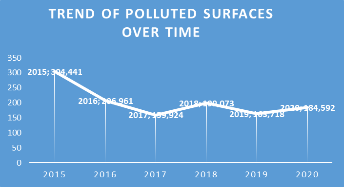
From the above results, we can deduce a regression in pollution due to hydrocarbons from 2015 to 2020. This drop is estimated at around 119.85 km², or a reduction of around 39.37% as mentioned above. Thus between 2016 and 2020 the spreading surfaces of hydrocarbon slicks from oil concessions vary between 150 and 200 km². Fig 4 shows the evolution of the surface area polluted by hydrocarbons in the region studied.

 

 

 

 

 

 

 

 

 

 

 

 

 

 

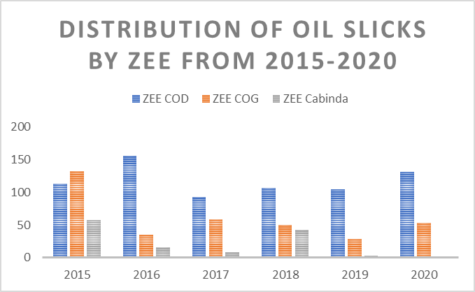
We also clearly see that the most recurrent and highest pollution areas are observed in the DRC's EEZ. In 2015 we observed around in the EEZ of the Democratic Republic of Congo (ZEE COD) a surface area of spread of hydrocarbon slicks of approximately 110 km² compared to 130 and 50 for the EEZ of the Republic of Congo (ZEE COG) and Cabinda. However, between 2016 and 2020, the pollution areas observed in the DRC are almost greater than 100 km², up to 150 km² in 2016 and in the case of the exclusive economic zones of the Republic of Congo and Cabinda, the pollution areas are almost less than 50 km². Fig. 5 shows the cumulative surface areas of oil spills by EEZ for each country.

 

                                              

 

 

 

 

 

 

 

 

 

 

 

 

 

 

5. Discussion

 

The results obtained show large areas of spreading of oil slicks which may be due to frequent and uncontrolled spills. During data collection we used 644 pieces of data. Depending on the number of data downloaded per year, the probability of detecting slicks is greater. Thus, the data collected in 2015 and 2016 are not very representative compared to that collected between 2017 and 2020. The observation that emerges is that this trend is decreasing year after year. To reduce margins of error in detection, we used a stochastic approach which consists of obtaining a large number of samples or data in order to optimize the detection of oil slicks, this approach was carried out in the framework of certain works such as those of (Najoui 2017; Amoussou 2018). A more detailed analysis shows that the DRC is the most impacted country. The EEZ of the Democratic Republic of Congo has a strong presence of oil slicks. We also observed that the average surface area covered by oil slicks is 117.6 km² in the DRC and 59.81 km² for Congo Brazzaville. However, some works, notably those of (Najoui 2022), have shown that the DRC had an average of low pollution areas (around 50 km²) compared to that of the Republic of Congo Brazzaville (250 km²) 2002 and 2012. We noted that the DRC has heavily polluted after 2015. From a general point of view, the results show a decreasing trend of around 8% corresponding to a reduction of around 97.4 km². This percentage is, however, put into perspective by the DRC which is an exception to the rule. Several potential avenues can explain this situation for this country. Firstly, the weakness of legislation in the face of the power of oil lobbies. Secondly, the insufficiency of controls by state authorities and finally thirdly, the obsolescence of production equipment leading to potential accidents. As we see in our results, the Congo Basin is strongly threatened by groundwater pollution. This threatening situation weighs on the preservation of coastal and marine ecosystems. In this area of preservation, scientific work has shown that when such phenomena occur, the presence time of hydrocarbons as a function of the volume spilled into the marine environment depends on its density (Wegener 2006). This work shows that for a density lower than 0.8 or between 0.8 and 0.85 the presence time could be expressed between 1 hour and 2 hours. These data differ slightly when it comes to light crude oil (density between 0.85 and 0.95) and heavy oil (density above 0.95), the dwell time could be estimated between a week and a year (Wegener 2006). These uncontrolled spills can often appear on coasts in the form of tar or foam, which cause numerous disruptions to coastal ecosystems and a reduction in the resilience of mangrove sites (Wegener 2006). Another consequence linked to this phenomenon is the threat to planktonic species, fish generally in the juvenile stage, marine birds whose soiling of their plumages is the most significant effect of this pollution, marine mammals which during their outings surface are left with damage to nasal tissues due to hydrocarbons (ITPFO 2013).

In order to reduce the risk of error in identifying slicks in the results we have just presented, we relied on the principle that oil spreads very quickly on the surface of the sea. About twelve hours after a spill, the slick can cover an area extending over several kilometres (PNIU, 2012). To enable us to map oil slicks effectively, we relied on the sensor characteristics of the Sentinel 1 satellite, which is capable of observing an area once every 12 days. By combining the orbital characteristics of Sentinel 1_A and 1_B, this gives us an exact repeat cycle of 6 days at the equator. With this approach, we believe we have considerably reduced the risk of duplicates in the same area. However, this probability is not zero, since throughout the drift of the slicks, there are changes in the content and shape of the oil slicks.

With regard to the methodology we have adopted, it is important to emphasise that failure to take into account factors such as wind speed, polarisation, incident angle, the effect of dielectric properties and the nature of oil slicks has a major influence on the process of detecting hydrocarbon products at sea. This is why we believe that any GIS modelling must take into account the states that a slick can experience.

6. Conclusion and perspectives

 

As underlined by Najoui (2017), radar sensors are commonly used in oil spill monitoring systems because of their well because of their proven detection capability. The emergence of new satellites that are more efficient with larger volumes of data makes automatic oil spill oil slick detection a necessity. However, oil slick detection is a multivariate phenomenon that depends on several factors. Multivariate phenomenon that depends on several parameters. The present work, which is a retrospective study, made it possible to highlight the phenomenon of pollution between 2015 and 2020. This study highlights that the maritime coast of the two Congos and Cabinda is exposed to numerous oil spills with large sprawling areas of up to 300 km2. However, this work remains to be improved by integrating not only the automatic approach into the processing of slick detection, but also models for deriving the objects identified using artificial intelligence. Such an approach would reduce the risk of redundancy in the process of identifying oil slicks during the scanning phases.

 

References

Amoussou, N. L. 2019. Data capitalisation and oil slick detection in the Gulf of Guinea from Envisat radar images 2002-2012. Sorbone2019.

 

Angiuli, E., F. D. Frate, and L. Salvatori. 2006. “Neural networks for oil spill detection using ERS and ENVISAT imagery.” In Proceedings of SeaSAR’06, 23-26 January 2006, Frascati, Italy, 1–6.

 

Brekke, C. and A.h.S. Solberg. 2005. "Oil Spill Detection by Satellite Remote Sensing." Remote Sensing of Environment 95 (2005): 1-13.

 

Chang, L., Z. S. Tang., S. H. Chang, and Yang-Lang, C. 2008. “A region-based GLRT detection of oil spills in SAR Images.” Pattern Recognition Letters 29 (14): 1915–23. doi:10.1016/j.patrec.2008.05.022.

 

Del Frate, Fabio, D. Latini, C. Pratola, and F. Palazzo. 2013. “PCNN for automatic segmentation and information extraction from X-band SAR imagery.” International Journal of Image and Data Fusion 4 (1): 75–88.

doi:10.1080/19479832.2012.713398.

 

EGE. 2022. Oil, the key to power and influence in the Gulf of Guinea. 2022.

 

ETOGA. 2023. Governance of Marine and Coastal Biodiversity in the Gulf of Guinea. University of Nice-Sophia Antipolis, 1-192.

 

Garcia-Pineda, O. 2009. “Spatial and temporal analysis of oil slicks in the gulf of Mexico based on remote sensing”. Texas A&M University.

Gasull, A., X. Fábregas, J. Jiménez, F. Marqués, V. Moreno, and M. A. Herrero. 2002. “Oil spills detection in SAR images using mathematical morphology.” In 11th European Signal Processing Conference (EUSIPCO 2002), 25–28. Toulouse, France. doi:10.1.1.81.3086.

 

Houndegnonto Odillon J. 2022. Analysis of thermohaline variations in the intraseasonal scales of the freshwater beds of the Goffe de Guinee. HAL Open Science, 13-185.

 

ITPFO. 2013. Technical Information Guide ,The Effect of Oil Pollution on the Environment. Cantebury: Impact PR & Design Limited. 2013

 

Kanaa, T. F. N., E. T. G . Mercier., V. P. Onana., J. M. Ngono., P. L. Frison., J. P. Rudant, and R. Garello. 2003. “Detection of oil slick signatures in SAR images by fusion of hysteresis thresholding responses.” In IGARSS 2003. 2003 IEEE International Geoscience and Remote Sensing Symposium. Proceedings (IEEE Cat. No.03CH37477), 4:2750–52. IEEE. doi:10.1109/IGARSS.2003.1294573.

 

Kounou Michel 2009. Oil and Poverty South of the Sahara: Analysis of the Foundations of the Political Economy of Oil in the Gulf of Guinea, Yaoundé, Clé, 2006, p. 21.

 

Liu, A. K., C. Y. Peng, and S. Y. Chang. 1997. “Wavelet analysis of satellite images for coastal watch.” IEEE Journal on Ocean Engineering 22 (1): 9–17

 

Malouana Biggie. 2022. Serious oil spill at the Cap Lopez terminal. Port-Gentil: Gabon Review.

 

Mbaki Esther Pabou. 2003. The Congo unarmed in the face of oil pollution. VertigO - la revue électronique en sciences de l'environnement [On line], Regards / Terrain, online 01 May 2003, accessed 01 December 2023..

 URL : http://journals.openedition.org/vertigo/4856 ;

 

Monde Afrique. 2022. Congo Brazaville under power lines, villages in the dark. 12 October 2022.

 

Najoui, Z.,   N.Amoussou.,  S. Riazanoff.,  G. Aurel, G., and  F. Frappart. 2022. Oil slicks in the Gulf of Guinea – 10 years of Envisat Advanced Synthetic Aperture Radar observations. Earth Syst. Sci. Data 14 : 4569–4588, https://doi.org/10.5194/essd-14-4569-2022, 2022.

 

Najoui, Z. 2017. Prétraitement optimal des images radar et modélisation des dérives de nappes d'hydrocarbures pour l'aide à la photo-interprétation en exploration pétrolière et surveillance environnementale,https://pdfs.semanticscholar.org/92b2/e8e06b49d7f31c0847c694f4b4f3bea41222.pdf?_ga=2.235046721.1549874629.1594648502-969427726.1594648502 (last access: 14 October 2022), 2017. 

Najoui, Z. 2022a. 100 geolocated oil spills in the Gulf of Guinea (1.0), Zenodo, https://doi.org/10.5281/ZENODO.6907743, 2022a. 

Najoui, Z. 2022b. Spatial distribution of oil slicks in the Gulf of Guinea between 2002 and 2012, Zenodo, https://doi.org/10.5281/ZENODO.6470470, 2022b. 

Najoui, Z., Riazanoff, S., Deffontaines, B., and Xavier, J.-P. 2018a. A Statistical Approach to Preprocess and Enhance C-Band SAR Images in Order to Detect Automatically Marine Oil Slicks, IEEE T. Geosci. Remote, 56, 2554–2564

https://doi.org/10.1109/TGRS.2017.2760516, 2018a 

 

Najoui, Z., Riazanoff, S., Deffontaines, B., and Xavier, J.-P. 2018b. Estimated location of the seafloor sources of marine natural oil seeps from sea surface outbreaks: A new “source path procedure” applied to the northern Gulf of Mexico, Mar. Petrol. Geol., 91, 190–201, https://doi.org/10.1016/j.marpetgeo.2017.12.035

Ngodi, E.: Gestion des ressources pétrolières et développement en Afrique, Présentation à la 11ème Assemblée générale du CODESRIA (6–10 December 2005), Maputo, Mozambique, 2005. 

Ndoutoume xxxxxx. 2010. Terrorism and piracy: what security for the seas of the Gulf of Guinea? FES, 159-182.

 

Ngoma Khuabi Camille. 2015. Corporate social responsibility and repair of ecological damage due to oil pollution in the coastal city of Moanda in the Democratic Republic of Congo. KAS African Law Study Library, 9-41.

 

Okafor-Yarwood, I.: The effects of oil pollution on the marine environment in the Gulf of Guinea–the Bonga Oil Field example, Transnatl. Leg. Theory, 9, 254–271, https://doi.org/10.1080/20414005.2018.1562287, 2018. 

 

Tchetchoua Tchokonte Severin. 2019. Oil Issues and Games in Africa: Study of the Chinese Oil Offensive in the Gulf of Guinea, Master's Thesis in Political Science, University of Yaoundé II, 2007-2009.

 

Ona Ona Jenifer Octavie. 2019. Sustainable management of fisheries resources in Central East Atlantic Africa: Cameroon-Congo-Gabon. Nantes: 19 December 2019.

 

PNIU. 2012. Behaviour and Fate of Hydrocarbons. Tunisia

 

Topouzelis, Konstantinos N. 2008. Oil spill detection by SAR Images: Dark formation detection, feature extraction and classification algorithms. Sensors 8 (10): 6642–59. doi:10.3390/s8106642.

 

Solberg, A. H. S., G. Storvik, R. Solberg, and E. Volden., 1999. Automatic detection of oil spills in ERS SAR images. IEEE Transactions on Geoscience and Remote Sensing 37 (4): 1916–24. doi:10.1109/36.774704

 

Wald Lucien, Jean-Marie Monget, & Michel Albuisson. 2010. Oil pollution in the Mediterranean as seen by the Landsat satellite. Hal Open Science, 61-68

 

Wegener Angela. 2006. Marine pollution, case study.